Running from the GUI¶

The HELIX desktop app exposes the same workflows as the Python API (Simulation.run() / Simulation.run_envelope()) plus matching, error studies, and orbit correction — all without writing code. This chapter is the short "how do I just run a simulation" walkthrough. For a full tour of every tab and panel see GUI overview.

Launching¶

In a Python environment with the linac_gen_gui package installed (or via the bundled .exe):

# From source (Linux / macOS / WSL):
PYTHONPATH=/path/to/Linac_Gen:/path/to/Linac_Gen/gui \
    python3 -m linac_gen_gui.interphase

# Windows .exe build:
HELIX.exe

The window opens on the Beam tab.

Path A — envelope or multi-particle run¶

The simplest "track a beam through a lattice and look at the σ plots" workflow.

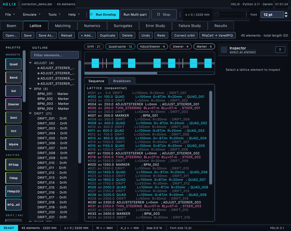
Lattice tab with the correction-demo lattice loaded

Lattice tab — toolbar (top), outline tree + filter (left), sequential lattice listing + element timeline (centre), inspector (right). The "Correct orbit" button sits in the toolbar between Undo/Redo and the summary text.

Lattice tab → Open… (or File → Open Lattice…, Ctrl+O). The filter accepts TraceWin .dat and MAD-X .madx / .seq files; projects open separately via File → Open Project…. The element timeline + outline tree populate.
Beam tab → set species, kinetic energy, RF frequency, current, distribution, and Twiss / emittance values. Hit Apply to commit — nothing else commits the form (no Tab-off), though the first Run pulls the form automatically if you haven't applied anything yet.

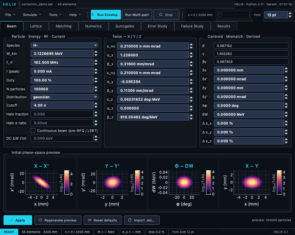
Beam tab — three fixed groups (Particle · Energy · RF · Current, Twiss — X / Y / Z, Centroid · Mismatch · Derived) and the four-panel initial-phase-space preview at the bottom. 3. Numerics tab (optional) → adjust integration step density, PIC grid resolution, or solver backend if the defaults don't fit your case. Most users skip this. 4. Toolbar → Run Envelope (Ctrl+R) for the fast σ-only pass, or Run Multi-particle (Ctrl+Shift+R) for the full macroparticle ensemble (with PIC space charge if a SpaceChargeConfig is configured). 5. Results tab → centroid / σ-x / σ-y / emittance / phase-space plots populate. The tab's only button is Import Results… (reload a saved run); saving figures or data happens per popup — open a card and press Ctrl+S or right-click for "Save plot…".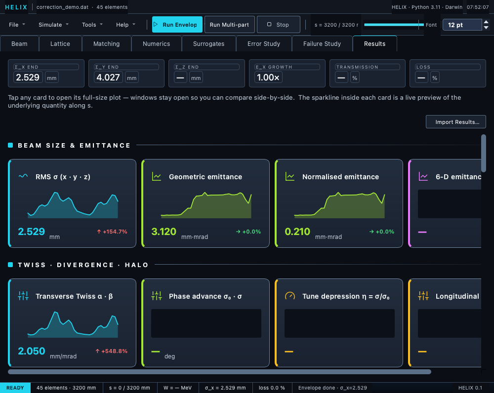

Results tab — KPI strip across the top (σ_x / σ_y / σ_z end, ε_x growth, transmission, loss); below that the result cards (RMS σ, geometric / normalised / 6-D emittances, Twiss, phase advance, tune depression, divergence, halo). Click any card to open the full-size plot; cards stay open side-by-side for comparison.

While a run is in flight the toolbar's s-label doubles as the progress readout — s = 3400 / 18957 mm · 18% — and the slider sweeps the lattice in real s (there is no elapsed-time display). Stop on the toolbar cancels a running worker cleanly without corrupting the partial recorder.

Path B — TraceWin matching (SET / ADJUST cards)¶

When the loaded .dat carries SET_* and ADJUST_* matching directives (or you've added them programmatically), the Matching tab picks them up automatically.

Load a lattice with SET_* / ADJUST_* cards (or use one of the worked examples in examples/matching/).
Matching tab → pick the algorithm and options in the Auto-Adjust panel. The variables, constraints, and bounds come from the .dat cards and are read-only in the GUI — to change a bound, edit the ADJUST card and reload. The Variables / Constraints tables are empty until a match has run.
Match → the matcher runs in the background and writes the converged values back onto the lattice. The default algorithm least_squares solves the system with Levenberg–Marquardt via SciPy; six others are available (differential_evolution, dual_annealing, gradient, cmaes, sequential_scan, bayesopt). The status line shows iteration count and baseline → final cost; the tables fill with per-variable values and per-constraint residuals.
After matching: Run Envelope to verify the σ trace meets your design intent. See Matching → Recipes for canonical patterns (achromat, beta-bumping, Twiss matching).

Path C — Monte-Carlo error study¶

Plant random errors per seed, track each, aggregate the ensemble.

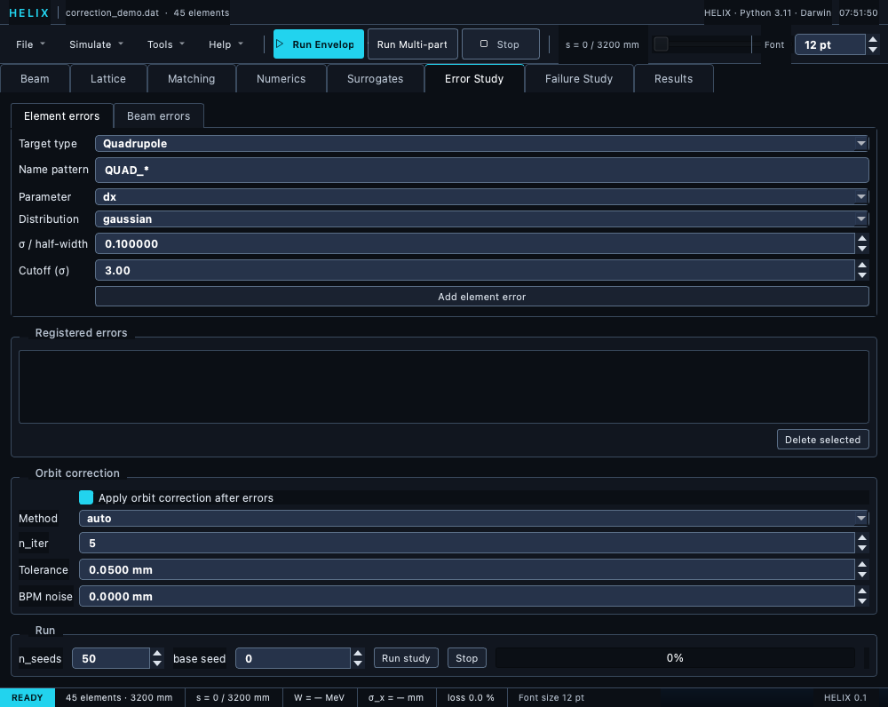
Error Study tab with a quad-dx spec ready to add and the
Orbit-correction group enabled

Error Study tab — element / beam-error forms at the top, list of registered errors below, the Orbit-correction group (with Method / n_iter / Tolerance / BPM-noise) in the middle, the Run group with n_seeds + progress bar at the bottom.

Lattice + Beam tabs → set up the deterministic baseline.
Error Study tab → element form → register one or more error specs. Pick target type (Quadrupole / Cavity / Bend / Solenoid), name pattern, parameter, distribution, σ or half-width, cutoff. Add element error. Repeat for as many specs as you want; register beam-input errors via the second form.
(Optional) Orbit correction group → tick Apply orbit correction after errors to run a correction pass per seed between error injection and tracking. See Errors → Orbit correction.
Run study → set n_seeds (start with 20-50) and hit go. Progress bar advances per seed.
Results tab → ensemble plots (mean ± σ envelope, per-seed centroid spread, transmission histogram).

Path D — Standalone orbit correction¶

A one-shot fix-up for a lattice that has steerers + BPMs (or ADJUST_STEERER + DIAG_POSITION cards).

Lattice tab → Open… the lattice.
Beam tab → confirm beam settings.
Lattice tab → Correct orbit toolbar button.
Summary dialog reports the chosen method, RMS-orbit before / after, and per-steerer kicks. Steerer bx_l / by_l are mutated in place; subsequent envelope / MP runs use the corrected values.

Full walkthrough + example numbers in Errors → Orbit correction → Path A.

Saving / restoring projects¶

A HELIX project (.lgproj) is a self-describing JSON snapshot of every user-settable GUI value (beam config, convergence config, correction settings, error specs) plus a path reference to the loaded lattice.

File → Save Project… writes a .lgproj next to your .dat.
File → Open Project… restores the entire GUI state in one click.
Auto-restore: on launch the GUI re-opens the most recent project if there is one, falling back to the last bare lattice otherwise (silently — no popup if it's missing). A project carries its own lattice reference, so the two never load together.

Automatic result dumps¶

Every completed run auto-writes two files into the calculation directory (File → Set Calculation Directory…):

<timestamp>_<run_type>.h5 — HELIX-native HDF5 schema.
<timestamp>_<run_type>.opmd.h5 — openPMD-1.1 (interop).

Either file can be reloaded later via the Results tab's Import Results… button.

Stopping / canceling¶

Long runs (multi-particle + 3-D PIC on a 256-m lattice) can take many minutes. Stop on the toolbar interrupts the worker thread between elements; the partial recorder is discarded and the results tab reverts to the previous run. Closing the window also cancels any active worker.