Worked example: Basic FODO¶

The simplest possible HELIX simulation: a 2-cell FODO with a 5 mA proton beam, multi-particle tracking with PIC space charge, plot σ_x vs s. 10 minutes from clone to plot.

Source¶

This walkthrough mirrors examples/basic_tracking.py. Run it directly:

python examples/basic_tracking.py

Lattice¶

A 2-cell FODO + RF gap:

from linac_gen.elements.drift import Drift
from linac_gen.elements.quadrupole import Quadrupole
from linac_gen.elements.rf_gap import RFGap
from linac_gen.core.lattice import Lattice

lat = Lattice()
for cell in range(2):
    lat.add(Quadrupole(name=f"QF_{cell}", length=100.0, gradient=+10.0))
    lat.add(Drift(name=f"D1_{cell}", length=200.0))
    lat.add(Quadrupole(name=f"QD_{cell}", length=100.0, gradient=-10.0))
    lat.add(Drift(name=f"D2_{cell}", length=200.0))
    lat.add(RFGap(name=f"GAP_{cell}", voltage=1.0, phase=-30.0,
                   frequency=352.21))   # voltage is in MV

Beam¶

from linac_gen.core.config import BeamConfig
from linac_gen.distributions.factory import create_beam

beam_cfg = BeamConfig(
    species="proton", energy=3.0, frequency=352.21,
    current=5.0, n_particles=10_000,
    distribution="gaussian", cutoff=4.0,
    emit_nx=0.25, emit_ny=0.25, emit_z=0.30,
    alpha_x=0.0, beta_x=2.0,
    alpha_y=0.0, beta_y=2.0,
    alpha_z=0.0, beta_z=1.0,
)
beam = create_beam(beam_cfg, seed=42)

Run¶

from linac_gen.core.config import SpaceChargeConfig
from linac_gen.core.simulation import Simulation

sc = SpaceChargeConfig(nx=32, ny=32, nz=32, kernel="cic")
sim = Simulation(lat, beam, space_charge=sc)
results = sim.run()

Plot¶

import numpy as np
import matplotlib.pyplot as plt

s_m = np.asarray(results.s) / 1e3
fig, ax = plt.subplots(2, 1, figsize=(10, 6), sharex=True)
ax[0].plot(s_m, results.sigma_x, label="σ_x")
ax[0].plot(s_m, results.sigma_y, label="σ_y")
ax[0].set_ylabel("σ [mm]"); ax[0].legend()
ax[1].plot(s_m, results.transmission)
ax[1].set_ylabel("transmission [%]"); ax[1].set_xlabel("s [m]")
plt.tight_layout()
plt.savefig("basic_fodo.png", dpi=120)

What you should see¶

Basic FODO σ_x and σ_y

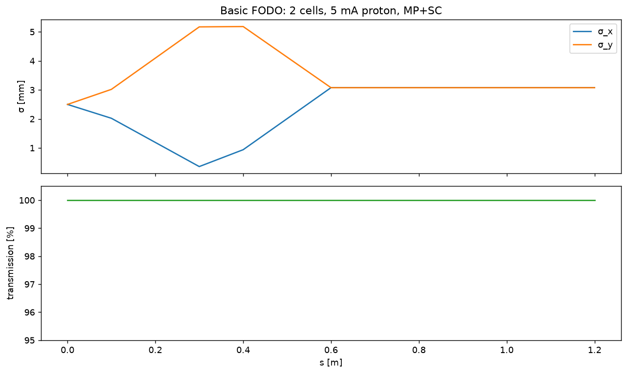
Figure 11.1 — Two FODO cells at right angles produce alternating σ_x focusing and σ_y focusing — both planes oscillate with the cell period. Transmission stays at 100 %. RF gaps subtract a small phase slip but for short lattices this is negligible.

Try this next¶

Modify and re-run to build intuition:

Crank up the current to 50 mA. Watch σ blow up — SC is significant.
Mismatch the input by changing beta_x to 0.5. Observe the σ_x oscillation amplitude is no longer matched.
Switch to envelope — replace sim.run() with sim.run_envelope() and watch the runtime drop 100×.

Cross-references¶

← GUI workflows · Continue to Envelope demo →