Matching tab

The Matching tab gathers three matching tools for the loaded lattice and beam: a Twiss dialog, a phase-advance analyser, and the card-driven auto-adjust matcher.

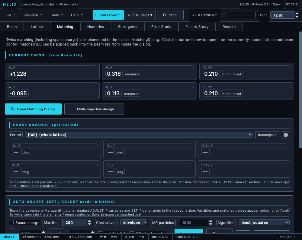
Matching tab — periods/KPIs, the σ₀ phase-advance panel, and the auto-adjust matcher controls.

Current Twiss

KPI cards at the top echo the input Twiss (α, β, ε) from the Beam tab — the starting point every tool uses.

Open Matching Dialog

Opens the classic Matching Dialog: it computes the periodic Twiss of a lattice (or section) and the space-charge-matched Twiss, and can write the result back into the Beam tab. Use it to find a matched input beam for a periodic structure.

Mode: Whole lattice vs FODO cell

The dialog's Mode dropdown offers two entries — "Whole lattice (periodic ring)" and "FODO cell → entrance (transfer line)" — switching between two distinct physical questions:

Mode	Physical question	Math
Whole lattice (find_periodic_twiss)	"What input Twiss, tracked once through the entire lattice, comes back to itself at the end?"	One-turn 6×6 transfer matrix M of the whole lattice → extract matched Twiss.
FODO cell (find_matched_input_twiss)	"There's a repeating sub-section. What Twiss do I inject at s=0 so the beam is matched to that sub-section's period by the time it arrives?"	Periodic Twiss of just the picked sub-cell, then back-propagated through the inverse of the front section to s=0.

When to use which

Whole lattice mode is for genuinely periodic structures:

Lattice type	Whole-lattice?	Why
Storage rings, synchrotrons, FFAGs	✓ Yes	The beam circulates; "one turn = lattice" is literally periodic.
Booster, main injector, collider arcs treated as rings	✓ Yes	Same reason.
A single FODO cell modeled in isolation, asking "what's the matched solution if this repeats forever?"	✓ Yes	Mathematically identical to a ring of one cell.
HWR / SSR / cryomodule cavities	✗ No	Accelerating: eigenvalues drift off the unit circle as βγ grows. Mathematically diverges.
MEBT, BTL, HEBT, dump lines	✗ No	Transfer lines — one-pass, not periodic. Use cell mode.
LEBT, RFQ	✗ No	Acceleration + non-periodic geometry breaks the assumption.

FODO cell mode is for everything else PIP-II-class: a transfer line or linac with a repeating sub-section inside it. Cell mode finds the matched injection Twiss — the entrance Twiss that lands the beam in periodic equilibrium by the time it reaches your chosen sub-cell.

Practical rule of thumb for PIP-II work

For every lattice in examples/pipii/* — HWR, SSR1, SSR2, LB650, HB650, MEBT, BTL — use FODO cell mode. Whole-lattice mode is there for ring lattices HELIX doesn't currently target.

If the cell mode auto-detection picks the wrong sub-cell or finds none (rare), use the --cell-start N --cell-end M flags on the CLI (or pick a different cell index in the GUI cell combo).

Cells with bends (BTL, dispersive arcs)

BTL and HEBT arcs include dipoles → there's dispersion in the matched beam. The zero-current find_matched_input_twiss only matches transverse betatron (α, β); it ignores dispersion. For arcs, use Compute SC-Matched Twiss even at zero or low current — it calls find_sc_matched_input_twiss which uses an 8-state formulation (α, β per plane + D, D' per plane) that matches dispersion together with the betatron Twiss.

Accelerating-section warning

When the chosen cell or whole lattice accelerates significantly (HWR cryomodule: βγ grows ~1.04× per period), the eigenvector / Wolski method emits a stderr line:

[matched-Σ] accelerating-section deviation 0.041 from unit circle
            (moduli=[0.9588, 0.9588, 0.9636, 0.9636]); matched Σ is
            the smooth approximation.

This is physics, not a numerical error — the matched Σ is the closest-to-periodic solution given the acceleration. Tolerance is ±15% off the unit circle; truly unstable lattices (>15% deviation) still raise.

Decoupled vs coupled lattices

The dialog auto-detects whether the transverse one-turn map is decoupled (block-diagonal x and y — typical for quadrupole-only FODO cells) or coupled (non-zero x↔y off-diagonals — solenoid sections, HWR-style cryomodules, skew quads).

• Decoupled: extracts standard Courant–Snyder α / β per plane from the 2×2 diagonal blocks. Fast and exact.
• Coupled: falls back to the eigenvector / Wolski method on the full 4×4 transverse map. Builds the matched 4×4 Σ from the two normal-mode eigenvectors and reports per-plane α / β as projections of that Σ (what x-only and y-only diagnostics measure), plus the two normal-mode phase advances μ₁ and μ₂.

When the coupled fallback fires, the log line is suffixed with [COUPLED -- normal-mode advances μ₁=…°, μ₂=…°; α/β are Σ projections] so you know the per-plane Twiss is the projection, not decoupled Courant–Snyder. This is the load-bearing fix for HWR cryomodule matching where the previous Twiss calculation refused to return (by design — the 2×2 trace is not the one-turn phase advance under coupling).

Multi-objective design…

The Multi-objective design… button opens a dialog that explores the Pareto trade-off between competing objectives (e.g. emittance growth vs exit energy) over the lattice's ADJUST knobs — distinct from the matcher, which drives a single scalar cost to zero. Tick ≥2 objectives, choose the algorithm (nsga2 genetic / qnehvi Bayesian) and cost solver, Run, then read the Pareto front off the scatter + table and Apply knee point to commit a balanced design. See Multi-objective design.

Phase Advance panel

Pick a period (LATTICE-card brackets are detected automatically, with a whole-lattice fallback) and the panel reports the channel tunes from the envelope phase probe: σ₀_model (bare) and σ_model (depressed, primary) with η_model = σ_model/σ₀_model as the tune-depression KPI, plus the beam Δμ_rms (secondary, with a tooltip caveat) from the latest envelope run. Coupled cells report the normal-mode tunes I/II; a "frozen-longitudinal" tag appears where the longitudinal fixed point is not solved. Validity notes surface when the beam is not matched (BMAG), when β is projected-only inside a coupled interior, or when sampling is coarse. See Phase advance & tune depression for the full definitions.

Auto-Adjust panel

Runs the lattice-driven matcher against the ADJUST_* variables and SET_* constraints already present in the loaded lattice — the variables and constraints are not entered in the GUI; they come from the .dat cards (see SET / ADJUST).

Controls (options row):

Control	Effect
Space charge	include space charge in the forward pass. Envelope cost-solver uses its linear-SC model; MP cost-solver uses the configured SpaceChargeConfig (Numerics tab).
Max iter	iteration cap (function evals for least_squares; generations for population algorithms)
Algorithm	optimiser — least_squares, differential_evolution, dual_annealing, cmaes, sequential_scan, gradient, or bayesopt
CMA-ES σ / popsize	initial step (fraction of bound width) and population size; enabled when algorithm is cmaes
no LS polish	skip the final least_squares refinement after the global search. Enabled for cmaes and bayesopt; greyed out otherwise.
BO physics prior	bayesopt only: warm-start an expensive MP match from the cheap envelope cost. Enabled when algorithm is bayesopt (effective with Cost solver = mp).
Cost solver	which forward pass computes the cost — envelope (fast linear, default) or mp (full PIC, physics-accurate, ~50–100× slower per eval).
MP particles	macroparticles per MP cost evaluation. Always visible, but enabled only when Cost solver = mp (greyed out otherwise). There is no seed spinbox.
Match	run the matcher in the background
Stop	cancel a running match. Lattice is restored to the best-cost x seen so far; the Variables table populates from that result.
Apply	write the matched values into the lattice + beam config; flags both as dirty so the close-without-save prompt warns you.
Save matched .dat	export the matched lattice to a TraceWin .dat

least_squares is local and fast. differential_evolution and dual_annealing are global searches — slower, and they require finite min/max bounds on every ADJUST card; if a bound is open-ended the run stops with an error naming the variable.

cmaes is the recommended general-purpose pick for ~5–30 variable matching problems. It learns the covariance matrix of "improving directions" and walks diagonally, which is much faster than coordinate descent on correlated knobs (cavity ke + phase pairs, quadrupole triplets). With refine enabled (default), CMA-ES chains a final least_squares polish from its best point.

sequential_scan is physics-aware coordinate descent — it walks elements in lattice order and brackets each ADJUST'd parameter (with FieldMap kb/ke/phase grouped). Clicking Match with this algorithm opens a setup dialog. Its controls:

Setup control	Effect
Element checklist	tick which ADJUST'd elements to scan (default: all)
Passes through lattice	full sweeps over the element list
Steps per parameter	bracket steps each parameter is walked per pass
Step size (fraction of bound width)	per-step displacement = this × (vmax − vmin)
Direction reversal	both grew (flip only when both transverse and longitudinal ε exceed the reference) or any grew (stricter)
Reversal reference ε:	the ε the reversal compares against — input beam ε (tight) vs seed exit ε (the unmatched lattice's exit ε; natural for intrinsic-growth ε-minimisation)
Beam loss (Reject any step that causes beam loss (HARD rule))	when ticked, any trial step whose transmission falls below the threshold is rolled back — best_x is not moved to it even if cost dropped — and the direction flips. Closes the gap where the matcher could "win" on ε by clipping halo. Requires Cost solver = mp (envelope mode tracks no losses; the control is inert there).
Loss-rejection threshold	transmission floor for that check — 100.00 % rejects any loss; 99.90 % tolerates sub-permille; enabled only when Beam loss is ticked

See the Sequential-scan section for the physics and when to use each combination.

bayesopt is Gaussian-process Bayesian optimisation (BoTorch) — the most sample-efficient global optimiser, reaching the optimum in the fewest forward passes. It is the right pick for expensive matches (set Cost solver = mp / tick Space charge) and multimodal / one-sided-constraint landscapes. Tick BO physics prior to warm-start an MP match from the cheap envelope cost. Like cmaes it chains a least_squares polish (untick no LS polish to keep it). It is not the default — for cheap linear-envelope matches least_squares / gradient reach the same optimum faster in wall-clock. See examples/ml_bayesopt/ for a runnable A/B convergence demo.

Step-by-step: a Bayesian-optimisation match

1. Load a lattice with ADJUST_* + SET_*/MIN_* cards and set the beam on the Beam tab → Apply.
2. In Auto-Adjust, set Algorithm → bayesopt. (This enables the BO physics prior checkbox, which only bayesopt unlocks, and the no LS polish checkbox, which is enabled for cmaes and bayesopt.)
3. Set Max iter = number of Bayesian iterations (≈ 20–40 is plenty; BO is sample-efficient).
4. For the expensive case — the one BO is for — set Cost solver → mp and tick Space charge, then tick BO physics prior. The prior only has an effect in this exact combination (bayesopt and Cost solver = mp); it warm-starts the slow MP match by first scouting the box with the cheap envelope cost. For a quick envelope match, leave Cost solver = envelope and the prior checkbox does nothing.
5. Leave no LS polish unticked to keep the final least_squares clean-up from the BO best (recommended).
6. Click Match. The live convergence dialog plots cost + εnx/εny/εnz per evaluation; Stop keeps the best point so far.
7. Review the Variables / Constraints tables, then Apply to write the matched values into the lattice + beam (flags the project dirty), or Save matched .dat to export.

gradient is a local search that replaces the finite-difference Jacobian with an exact one from differentiable tracking. It covers SET_TWISS / SET_SIZE matching of quad / solenoid / dipole knobs — and, with Space charge ticked, matches through the non-linear PIC space charge (a macro-particle bunch tracked by the differentiable PIC step tracker). It needs an all-linear lattice — drift / quad / solenoid / dipole, no RF or field maps; outside that it stops with a clear message telling you to switch back to least_squares. For matching sections with several knobs the exact Jacobian also runs faster than the finite-difference one.

Live convergence dialog

While the match runs, a non-modal Match Convergence dialog stays on top showing:

• Cost trace — current cost + monotone-decreasing best-so-far on a log-Y axis vs evaluation index.
• Emittance trace — εnx, εny, εnz vs evaluation index on a linear-Y axis so you can watch the actual physics metric, not just the optimiser's cost.
• Live values panel — current εnx/εny/εnz, W_kin at exit, and (for sequential_scan only) the element + ADJUST attr being scanned, pass/step counters, scan direction.

Closing the dialog does not stop the match; that's the Stop button's job.

Beyond the convergence dialog, any Results-tab popup with its live match preview checkbox ticked (e.g. the Centroid popup with the diagnostic goal-orbit overlay) re-plots the matcher's current iterate about once per second during the run — see Results tab.

After a run

Two read-only tables fill in:

• Variables — name, initial value, matched value, bounds.
• Constraints — name, RMS residual, notes. Every SET_* / MIN_* card in the lattice gets a row here, including the soft-penalty cards MIN_EMIT_GROWTH, MIN_EMIT_4D_GROWTH and MIN_TRANSMISSION — e.g. a MIN_TRANSMISSION 99.9 50.0 card shows up as a MIN_TRANSMISSION row whose residual is non-zero only when the beam drops below 99.9 % transmission (and is meaningful only with Cost solver = mp, since envelope mode tracks no losses). Read its residual to confirm the match didn't buy a low emittance by clipping the beam. See SET / ADJUST cards.

…and the status line shows OK / FAILED / Cancelled — best of run followed by — N iters, cost baseline_cost → final_cost, T s. The baseline cost is the cost at the unmatched x0, so you can see at a glance whether the match actually improved things.

Workflow

1. Load a lattice that contains ADJUST_* / SET_* cards.
2. In Auto-Adjust, pick the algorithm and (optionally) Space charge.
3. Click Match and watch the status line.
4. Review the Variables / Constraints tables.
5. Click Apply to commit, or Save matched .dat to export.

The algorithm choice and Max-iter are session settings — they are not saved in the .lgproj project file.

Cross-references

• Matching → Overview
• SET / ADJUST cards
• Matching Python API
• Worked example: matching walkthrough

← Numerics tab · Continue to Surrogates tab →