Results tab
The Results tab is your post-tracking dashboard. After a run, diagnostic data is grouped into "tiles" (cards) by topic; click any tile to open a popup with the full plot + numerical summaries. Popups stay open side-by-side for comparison.
Nearly every tile carries a live sparkline thumbnail and an end-value + trend footer. Most read a recorded array directly; the rest derive their series (cumulative phase advance, per-cell tune depression and Hofmann ratio from the probe, dispersion and σ(Δp/p) from the Σ-matrix, beam power, centroids) — and the LATTICE PARAMETERS tiles read the loaded lattice itself, so they render before any run and update when the lattice changes. A tile shows "—" only when its quantity genuinely doesn't exist yet: the per-cell tune tiles need a probe-bearing run and a declared periodic structure (an aperiodic whole line has no tune), the halo / IBS / stripping tiles need a multi-particle H⁻ run, and the phase-space / field-map / matrix tiles have no 1-D curve to preview. The footprint tile stays plain until you compute one in its popup.
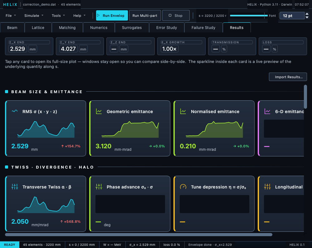
Results tab after an envelope run — KPI strip on top, tile sections with live sparklines below.
KPI strip
Across the top, six always-visible KPI cards summarise the latest run at a glance: σ_x end, σ_y end, σ_z end (mm), ε_x growth, transmission (%), and loss (%).
Import Results…
The Import Results… button loads a previously saved run — a
HELIX-native .h5 or an openPMD .opmd.h5 (auto-detected) — and
feeds it through the same path a live simulation uses, so the KPI
cards, sparklines, and every popup re-populate from the on-disk
arrays. The file dialog opens in the configured calculation
directory, where every run's auto-saved dumps land (see
Running → GUI).
Tile sections
Nine section headers, top to bottom:
- BEAM SIZE & EMITTANCE — RMS σ (x · y · z), geometric emittance, normalised emittance, 6-D emittance.
- TWISS · DIVERGENCE · HALO — transverse Twiss α · β, phase advance σ₀ · σ, tune depression η = σ/σ₀, Hofmann stability chart, tune footprint (frozen SC), longitudinal Twiss, divergence σ_x' · σ_y', peak excursion X / Y_max, halo parameter H_x · H_y. The phase-advance and tune-depression popups plot the channel tunes (σ_model, primary) with the beam Δμ_rms as a secondary series; the Hofmann and footprint tiles are the two space-charge diagnostics described below.
- ENERGY · KINEMATICS — energy · γ · transmission, beam power, 4-D invariant ε_4D, eigenemittances ε₁ · ε₂ · ε₃.
- LOSSES · TRANSMISSION — loss profile, aperture-profile losses, loss power (W/m · W/cm²), intra-beam stripping (H⁻), magnetic stripping (H⁻), and the error-study ensemble tile.
- CENTROID · DISPERSION — centroid ⟨x⟩ · ⟨y⟩ · ⟨φ⟩,
longitudinal offset Δφ_s · ΔW_s, dispersion D_x · D_y, and
σ(Δp/p) along s (the momentum-spread plot; see
σ(Δp/p) tile below).
The dispersion popup plots the statistical dispersion of the
tracked beam —
D_u = ⟨u·δ⟩/⟨δ²⟩from the Σ-matrix cross terms, which includes space charge and any seeded input dispersion — and a Transfer-matrix model checkbox overlays (dashed) the dispersion of the lattice itself: the unit energy-offset ray propagated by the element transfer matrices, seeded from the Beam tab's input dispersion, computed in a background worker (field-map matrices are RK4-integrated on first use, so the first overlay on a long linac takes tens of seconds; later toggles are instant). On a static, space-charge-free line the two curves coincide exactly — where they split, the difference is beam physics (space charge, nonlinearity), not machine optics. When the loaded lattice carries diagnostic-matching targets (DIAG_POSITIONoperands or a loaded BPM-targets file), the centroid popup overlays the goal orbit as hollow points at each BPM and a banner reports the achieved-vs-goal rms gap per plane — the direct "how close are we to what the diagnostics asked for" view. Envelope results carry a real first moment too, so the same achieved-vs-goal banner appears for both tracking modes; only results from sources that genuinely carry no centroid (e.g. loaded archives) fall back to a note saying so.
Every popup carries a live match preview checkbox (top-right, off
by default). Ticked, the popup re-plots the Matching tab's current
iterate about once per second while an optimization runs — watch the
orbit walk onto the goal points as the fit converges — and its title
shows LIVE match iter N. When the match ends the popup snaps back to
the committed results. Unticked popups ignore the stream entirely.
This is separate from end-of-run refresh, which is always on: every
visible popup updates whenever a normal run completes, regardless of
the checkbox.
* PHASE SPACE · DIAGNOSTICS — Phase space (4-panel) (the
full phase-space view at any snapshot marker), density-vs-s
heatmap, BPMs, field-map viewer (2D + cuts), cavity TTF T(β).
The phase-space popup's **Beam parameters** toggle (2026-07) swaps
the four density panels for a full parameter table of the
*selected* distribution — location, species/mass/charge, beam
current, reference particle (s, W_kin, β, γ, βγ, φ_s), centroid,
RMS sizes (incl. derived σ_z and σ_δ), Twiss for **all three
planes** (α_z/β_z in the internal (Δφ, ΔW) convention — α_z =
−TraceWin's, β_z in deg/MeV), geometric / normalized / 4-D /
eigen-emittances, Wangler halo, and per-coordinate max extents.
The table follows the location selector, and ++ctrl+s++ exports it
like any other popup data.
- LATTICE PARAMETERS — per-element field/optics scalars read off the lattice itself; see Lattice-parameter field plots below.
- CROSS-CHECKS · COMPARE — compare with TraceWin partran output.
- ADVANCED · MATRIX VIEWERS — Σ matrix (6×6), transfer matrix (6×6), SC convergence. These three cards don't open popups of their own: the Σ-matrix and transfer-matrix cards route to the Tools → Show Sigma Matrix… / Show Transfer Matrix… dialogs, and the SC-convergence card jumps to the Numerics tab, where the convergence scans live.
Raw vs Dispersion-corrected toggle
Six popups expose a Display dropdown at the top with two options:
- Raw (includes dispersion) — the σ-matrix entry as recorded.
In dispersive regions (arcs, RF-coupled sections, solenoid HWR /
SSR cryomodules with non-zero Σ[i,5] cross terms) this includes
the dispersive contribution
D · σ_δ. - Dispersion-corrected (betatron only) — the pure-betatron part, obtained by subtracting the Schur complement on the σ-matrix energy block:
From these, σ_x,β = √Σ_β,(0,0), ε_x,β = √(Σ_β,(0,0)·Σ_β,(1,1) − Σ_β,(0,1)²), α_x,β = −Σ_β,(0,1)/ε_x,β, β_x,β = Σ_β,(0,0)/ε_x,β.
Which popups carry the toggle:
| Popup | Raw display | Dispersion-corrected display |
|---|---|---|
| RMS σ (σ_x, σ_y) | recorded sigma_x, sigma_y |
√Σ_β,(0,0), √Σ_β,(2,2) (σ_φ stays raw — already in the energy plane) |
| Emittance (ε_x, ε_y, ε_t 4-D) | recorded emit_x, emit_y, emit_4d |
√det(Σ_β,2×2) per plane, √det(Σ_β,4×4) for 4-D (ε_z stays raw) |
| Normalised emittance | emit_nx, emit_ny |
ε_β · (βγ) per plane |
| Twiss (α, β) | alpha_x, beta_x, alpha_y, beta_y |
α_β, β_β from Σ_β,2×2 |
| Divergence (σ_x', σ_y') | √Σ_11, √Σ_33 | √Σ_β,(1,1), √Σ_β,(3,3) |
| Peak excursion (X_max, Y_max) | particle-tracked x_max / fallback 5·σ_x | fallback path uses 5·σ_β; MP-tracked x_max is the raw truth in both modes |
When to use each:
- Raw for aperture / loss studies — what actually hits the wall.
- Dispersion-corrected for matching diagnostics — the design β·ε comparison only holds for the pure-betatron part. In any dispersive section the raw σ disagrees with the design β by the dispersion-induced inflation; the corrected view removes it so the measured optics matches the design intent.
Edge case — DC beam / zero energy spread: when Σ[5,5] ≤ ε, the dispersive contribution is zero by construction, so the helper returns the raw entries unchanged. No NaN, no zero-division.
Cross-references:
σ(Δp/p) tile— the related plot of the beam's momentum spread along s; the same σ_W and reference β, γ that go into the σ(Δp/p) tile drive the Schur-complement correction here.- Dispersion (D_x · D_y) popup — explicit dispersion functions; the disp-corrected σ_x and Dispersion together let you read off the dispersive contribution σ_x² − σ_x,β² = D_x²·σ_δ² for internal-consistency checks.
σ(Δp/p) tile — RMS momentum spread along s
Computed from the recorded RMS energy spread σ_W(s) and the
reference particle's β, γ:
This is the inverse of the conversion the Dispersion D_x/D_y tile applies internally, so the two are mathematically consistent.
Typical values for a proton beam in the PIP-II energy range (σ_W ≈ 10 keV at 2-10 MeV): σ(Δp/p) of order 10⁻³ to 10⁻⁴.
What to look for:
- Adiabatic damping through accelerating sections: as the beam picks up energy, β²γ·m₀c² grows, so σ(Δp/p) shrinks even though σ_W stays roughly constant. A jump in σ(Δp/p) at a cavity boundary indicates real longitudinal mismatch (not just acceleration).
- Longitudinal acceptance for downstream RF buckets — the acceptance is usually quoted in dp/p, not σ_W; this plot lets you read it off directly.
- Dispersion-driven beam size: in arcs (BTL), σ_x picks up a
contribution
D_x · σ(Δp/p); reading both off their respective tiles tells you whether dispersion or betatron motion dominates.
Source: _DpPRmsPopup in gui/linac_gen_gui/interphase/tabs/results_tab.py
(uses the same sigma_w / ref_beta / ref_gamma / mass_mev
fields as the Dispersion popup, with the same fallback for
mass_mev when it's not in the results).
Space-charge diagnostics — Hofmann chart & tune footprint
Two tiles in TWISS · DIVERGENCE · HALO open the space-charge diagnostics built on the channel tunes (full theory: Hofmann stability & tune footprint):
-
Hofmann stability chart — opens with the exact per-cell (k_z/k_x, k_x/k_0x) trajectory (instant, from the pre-computed phase-probe maps). Compute chart then solves the corrected anisotropic l=2/3/4 KV dispersion relations off-thread and renders the γ/ν₀ₓ growth-rate heatmap at the trajectory's median ε_z/ε_x, with each cell classified: green = valid + stable, red = flagged (γ/ν₀ₓ > 0.01 inside the S² ≤ 10 gate), grey hollow = extrapolated (S² > 10), amber ring = fold risk. Optional toggles add per-cell Monte-Carlo
P(unstable)and the indicative legacy m/n bands. -
LEBT compensation (SCC) — for DC/continuous results only: choose gas and pressure (log slider 10⁻⁷–10⁻⁴ mbar), solver mode (Computed Poisson–Boltzmann balance / Assumed η), trapped-ion temperature, end taper and build-up time, then Compute for f_c(z), φ(z), τ_scc(z) and gas-survival profiles — plus suggested
SPACE_CHARGE_COMPfactors with Export cards and a confirm-gated Apply to lattice… (full theory: LEBT compensation). - Tune footprint (frozen SC) — press Compute footprint to re-track the selected cell off-thread with a frozen matched-beam field; the scatter shows each particle's (μ_x, μ_y) coloured by launch amplitude, with the core tune and spread in the caption.
For multi-particle results (no probe maps), the tune-depression popup offers a Compute channel model button — a companion envelope probe at the current Beam-tab config that fills the model curves next to the MP beam markers; the Hofmann chart reuses the same cached probe.
Lattice-parameter field plots
The LATTICE PARAMETERS section plots a single scalar per element, read from the lattice (design values) rather than the tracked beam — one stem at each element's mid-point. Each shows a centred "no data" message when the lattice has no element of that type.
| Tile | Quantity | Elements | Units |
|---|---|---|---|
| Quadrupole gradient | G |
quads | T/m |
| Quadrupole ∫G·ds | G·L |
quads | T |
| RF voltage (V₀) | \|ke\|·∫\|E_z\|dz/\|norm\| (or lumped voltage) |
RF gaps, cavity field maps | MV |
| Peak E_acc | peak axial accelerating gradient | cavity field maps | MV/m |
| Peak solenoid |B_z| | on-axis peak field | solenoids, magnetic field maps | T |
| Solenoid ∫B²·dz | integrated B_z² — focusing strength | solenoids, magnetic field maps | T²·m |
| Dipole field |B| | Bρ/\|ρ\| (hard-edge) |
dipoles (BEND) |
T |
| Dipole ∫B·dl | B·L = Bρ·θ |
dipoles (BEND) |
T·m |
| Floor plan (survey) | design-trajectory geometry | whole lattice | m |
| Synchronous phase | φ_s |
RF / field-map elements | deg |
∫B²·dz is the energy-independent measure of a solenoid's transverse
focusing strength: the solenoid focusing parameter is
(1/2Bρ)²·∫B_z²·dz, so this integral captures the lens shape independent of
beam energy. It is computed for both solenoid representations — a lumped
SOLENOID (hard-edge uniform field → B₀²·L) and a magnetic field map
(trapezoidal integral of the on-axis B_z(z)² profile, scaled by
kb·scale/norm). RF cavities (field maps with an E channel) are excluded.
The dipole tiles are the one lattice-parameter pair that needs the beam:
a BEND card stores only geometry (bend angle θ and curvature radius
ρ), so the field is B = Bρ/|ρ| at the beam rigidity. After a run
the rigidity is taken per element from the run's reference energy (exact
through accelerating sections); before any run it uses the beam-config
entrance energy — exact for fixed-energy transfer lines. Without a beam
configuration the tiles show the placeholder rather than a guess. Since
θ is fixed by the card, ∫B·dl = Bρ·θ — the field-integral tile is the
design invariant that stays constant when a dipole is shortened at fixed
bend angle.
Floor plan (survey) walks the reference orbit through the lattice in
3-D and draws the design trajectory: a top view (x–z, aspect-locked,
horizontal dipole arcs highlighted) and a side view (y vs path length
s, vertical dipole arcs highlighted), with entrance/exit markers and a
summary line (path length, Σ|θ|, dipole counts, exit coordinates). Pure
lattice geometry — no run required; a straight lattice draws a straight
line. Sign conventions: positive horizontal bend angle curves toward
+x, positive vertical angle (hv=1) toward +y; MAD-style negative
drifts step backward.
Popup details
Each tile popup shows:
- The plot (zoomable, toggle log/linear).
- An optional lattice-element strip along the s-axis — a colour-coded impression of the lattice, toggled by a checkbox and drawn without obscuring the curves.
- A numerical summary at top (means, ranges, percentile values).
Saving from a popup: press Ctrl+S or right-click for the context menu ("Save plot… (Ctrl+S)") — there are no dedicated save buttons. One dialog covers both data and image exports: pick a data format (CSV / NumPy .npz / JSON / HDF5) to write the plotted arrays, or an image format (PNG / JPEG / SVG / PDF) for the figure itself. Ctrl+W or Esc closes the popup.
Tile availability
The tile grid is static — every card is always shown, and cards whose data is missing simply open an empty/"no data" view. The one exception is Intra-beam stripping (H⁻): the card is disabled unless the beam species is H⁻, and its tooltip explains how to switch (Beam tab → Species → H- → Apply). Loss power needs a multi-particle run (envelope mode records no per-particle losses) and a non-zero beam current — it says so in place rather than drawing an empty plot, and its exit-plane W/cm² map additionally needs the final distribution, so it fills on live MP runs while a reloaded file keeps the W/m profile. Eigenemittances are always recorded — there is no flag to enable them. The error-study ensemble popup fills only after an Error Study run, and the phase-space popup needs snapshot markers (or Numerics → "Snapshot every N") to have data.
Exporting to openPMD
The toolbar's Export openPMD output… action writes the most
recent run to an openPMD-1.1 HDF5 file (*.opmd.h5) — a portable
interchange format readable by openPMD-aware tools. See
Reading results → openPMD.