Tracking modes
HELIX offers three complementary simulation modes. Picking the right one is the single biggest decision for any HELIX run — wrong choice either wastes hours or gives misleading results.
TL;DR — when to use which
| Goal | Mode | Speed | Output fidelity |
|---|---|---|---|
| Match Twiss / scan parameters | Envelope | fast | RMS only |
| Predict transmission, halo, loss | Multi-particle + SC | slow | full |
| Pre-RFQ continuous (DC) beam | Sacherer ODE or MP+2D-DC | medium | RMS or full |
| Linear-optics sanity check | Envelope no-SC | fastest | RMS only, ignores SC |
| Tolerance / error ensemble | Envelope (cheap) or MP (slow but accurate) | varies | RMS / full |
If unsure, run envelope first to verify Twiss / focusing strengths, then MP+SC for the production result.
The three modes
1. Envelope (RMS) tracking
linac_gen.tracking.envelope.EnvelopeSolver propagates the 6×6
σ-matrix element-by-element. Space charge is a thin defocusing
lens built from the Lapostolle / Wangler uniform-triaxial-ellipsoid
model with rms-equivalent semi-axes (√5 σ_x, √5 σ_y, √5 γ σ_z) and
Maxwell depolarisation factors (Carlson R_D elliptic integral).
It also propagates the beam centroid (first moment) alongside Σ —
seeded from the beam's centroid offsets and driven by steerer kicks,
dx/dy/tilt misalignment feed-down, dispersion and freq-jump
rescales — so envelope results expose the same centroid arrays the
MP recorder does (orbit plots, diagnostic matching, orbit correction
all work in envelope mode). Linear space charge does not move the
centroid (the beam's own field is centred on it — TraceWin's
approximation too), and particle loss is still invisible: transmission
observables remain MP-only.
Pros:
- 20–100× faster than multi-particle.
- Deterministic — no shot noise.
- Smooth gradients for matching / optimisation.
Cons:
- No halo, no loss, no non-Gaussian information.
- Linear in σ — wrong for strong nonlinear regimes (mismatched transport, large dispersion-energy coupling).
from linac_gen.tracking.envelope import EnvelopeSolver
from linac_gen.core.lattice import Lattice
from linac_gen.core.particle import PROTON
from linac_gen.core.reference import ReferenceParticle
from linac_gen.elements.drift import Drift
from linac_gen.elements.quadrupole import Quadrupole

# A small FODO to track through:
lattice = Lattice()
for c in range(2):
    lattice.add(Quadrupole(name=f"QF_{c}", length=100.0, gradient=+10.0))
    lattice.add(Drift(name=f"D1_{c}", length=200.0))
    lattice.add(Quadrupole(name=f"QD_{c}", length=100.0, gradient=-10.0))
    lattice.add(Drift(name=f"D2_{c}", length=200.0))

ref = ReferenceParticle(species=PROTON, w_kin=2.5, frequency=162.5)
initial = dict(
    emit_x=0.21 / ref.bg, alpha_x=1.23, beta_x=0.32,
    emit_y=0.21 / ref.bg, alpha_y=-0.1, beta_y=0.11,
    emit_z=0.06,           alpha_z=0.0,  beta_z=819.0,
)
solver = EnvelopeSolver(lattice, ref, initial, current=5.0)
results = solver.run()
print(results.sigma_x[-1])
See full reference: Python API → EnvelopeSolver.
2. Multi-particle (MP) tracking
linac_gen.tracking.tracker.Tracker propagates a macroparticle
ensemble. Each element exposes a track(beam) method; thin elements
apply momentum kicks, thick elements integrate via 6×6 transfer
matrices or a substepped field push (for field maps). A field-free
drift is pushed once unless space-charge kicks, sub-step diagnostics
or the bunch-train phase fold need its sub-steps
(StepConfig.drift_single_push, default on; losses inside such a
drift are located exactly on the particle's straight line).
Without space charge, MP tracking is exact for its element class (matrix elements: linear; 1-D/2-D field maps: first-order midpoint kick-drift; 3-D field maps: KD or DKD, selectable — only DKD is symplectic).
Pros:
- Captures halo, loss, non-Gaussian behaviour.
- Produces full Σ-matrix and per-particle phase space at any s.
- Required for transmission, aperture loss, error studies.
Cons:
- Slower (typical: 100s for a 256m lattice with 5000 particles).
- Statistical noise floor ≈ 1/√N on σ.
3. Multi-particle + space charge (PIC)
Same Tracker but with a SpaceChargeConfig that activates the
PicSolver. At every integration step, the PIC cycle:
- Boost particles to the beam rest frame on z (γ on z only).
- Deposit charge on a 3-D Cartesian grid (CIC or TSC kernel).
- Solve Poisson via doubled-grid Hockney FFT (open BCs).
- Gather E-field back to particles.
- Apply transverse + longitudinal kicks directly to the lab-frame x′/y′/ΔW (the boost back is folded into the β²γ² kick factor; the reference particle is never modified).
from linac_gen.core.config import BeamConfig, SpaceChargeConfig
from linac_gen.core.simulation import Simulation
from linac_gen.distributions.factory import create_beam

beam = create_beam(BeamConfig(current=5.0, n_particles=2000), seed=42)

sc = SpaceChargeConfig(
    nx=64, ny=64, nz=64,        # grid resolution
    grid_extent=5.0,            # ±5σ box
    kernel="tsc",               # quadratic 27-cell deposition
    green_kind="igf",           # Integrated Green Function
    use_gpu="auto",             # "cpu" / "gpu" / "auto"
)
sim = Simulation(lattice, beam, space_charge=sc)
results = sim.run()
For details on PIC kernels and convergence guidance see Space charge → PIC solver and Convergence guide.
DC (continuous-beam) modes
Pre-RFQ LEBTs operate on a continuous beam — there's no bunching yet, so the longitudinal coordinate is undefined. HELIX has two DC-aware paths:
Sacherer ODE solver
linac_gen.tracking.sacherer solves the continuous-beam envelope
equation:
with generalised perveance K = qI / (2π ε₀ m c³ (βγ)³) and a focusing function κ(s) read off element-by-element. Scope: drifts, hard-edge quadrupoles, 1-D / 3-D solenoid field maps. RF cavities and acceleration are out of scope.
2-D analytic DC kick (in MP mode)
linac_gen.pic.pic_solver.kick_continuous_2d applies the closed-form
transverse kick for a uniform-density elliptical-cylinder beam.
Activated automatically when the beam is continuous (Beam.continuous
== True). Faster than 3-D PIC, matches TraceWin's continuous-beam
formula.
For full DC-mode coverage see DC mode and LEBT DC worked example.
Decision matrix
| Question | Envelope | MP no-SC | MP + 3D PIC | Sacherer ODE | MP + 2D DC |
|---|---|---|---|---|---|
| Bunched (post-RFQ) beam? | Yes | Yes | Yes | No | No |
| Continuous (pre-RFQ) beam? | Yes (ε_z=0) | No | No | Yes | Yes |
| Need halo / loss? | No | Yes | Yes | No | Yes |
| Need transmission? | No | Yes (aperture) | Yes | No | Yes |
| SC effects matter? | rough | No | Yes | Yes | Yes |
| Need fast iteration? | Yes | Partly | No | Yes | Partly |
| Used in matcher? | Yes (default) | No | occasional | No | No |
Performance reference
A 256-m PIP-II lattice (mebt+hwr+ssr1+ssr2+lb650+hb650, 1763 steps), 5 mA H⁻ beam, 5000 macroparticles, 48³ grid, TSC kernel, on a modern laptop:
| Mode | Wall time |
|---|---|
| Envelope, no-SC | ~5 s |
| Envelope, SC | ~10 s |
| MP, no-SC | ~6 min |
| MP + 3D PIC SC | ~9 min |
The envelope solver is the right tool for matching and parameter sweeps; multi-particle is the right tool for the production answer.
Backward tracking
All three modes above walk the beam downstream. HELIX can also walk a
distribution backwards — from the exit of any element range to its
entrance — with backtrack_distribution (multi-particle) and
backtrack_envelope (RMS σ-matrix). Two workflows:
- Reconstruction — a measured (or exported) distribution at a
downstream point, e.g. a
.dstat a diagnostic station, walked upstream to recover the distribution that entered the line; - Design targeting — a desired exit distribution backtracked to find the required input, then validated by a forward re-run (the classic backward → forward closure loop).
How it works
Each forward operation Φ is undone by applying its exact algebraic
inverse Φ⁻¹ in reverse element / sub-step order (a drift the forward
tracker pushed once is undone with one inverse map — the backtracker
evaluates the same drift_single_push rule) — no coordinate flips,
no field-sign games, and every mid-walk diagnostic (σ, ε, Twiss) stays
directly physical. Matrix inverses use a true inv(M) (HELIX matrices
in mm/mrad/deg/MeV are not symplectic — RF adiabatic damping sits on
the diagonal — so the cheap symplectic inverse would be wrong at every
accelerating element).
The reference particle is never advanced in reverse. Instead the
design reference is replayed forward once over the range, recording
energy / phase / frequency / SC-compensation at every element boundary
(the replay table); the backward walk restores the reference from the
table at each boundary. SET_SYNC_PHASE cavities calibrate during the
replay with normal forward semantics and the calibration is reused.
Space-charge kicks depend only on particle positions, which the inverse
of each Strang half-map recovers — so the backward bundle
inv(M₂) → SC subtracted → inv(M₁) undoes the forward
M₁ → SC added → M₂ kick-for-kick, with the same kernels. This is
exact per step, and a short space-charge range closes to ~1e-14.
Over a long space-charge-dominated line it is not exact per particle:
the PIC field solve (float FFT deposit → solve → interpolate) is not
bit-reversible, and the tiny seed error is amplified by the collective,
effectively-chaotic space-charge dynamics through the ~10³ kicks of a
full linac section. The recovered beam moments stay accurate —
σ, ε and Twiss close to ~0.2–2.4 % over the whole MEBT+HWR at 5 mA — but
individual particle trajectories diverge (~0.14 mm median at that
scale). Under strong space charge, backtracking reconstructs the
beam, not a per-particle time-reversal (see the space-charge row
below).
What cannot be undone
| Limitation | Behaviour |
|---|---|
| Aperture losses | non-invertible — no cuts are applied backward; a warning notes the reconstruction covers survivors only |
| Field maps (cavities, solenoid maps) | undone exactly by default (field_map_mode="rk4"): each forward kick–drift step is closed-form invertible, and a zero-particle replay of the literal tracker schedule supplies bit-identical per-step references and SET_SYNC_PHASE calibration — full-MEBT round trips close at ~1e-13. field_map_mode="linear" keeps the v1 fitted-matrix inverse (~2 % through strong bunchers); RFQ cells and surrogate-driven elements always fall back to it |
| Quadrupole g3–g6 multipole content | undone exactly (position-only kicks re-applied with the opposite sign at the same positions — an IEEE-exact subtraction) |
| Fixed-grid PIC space charge | a fresh backward solver cannot rebuild the forward run's frozen grid — reuse the forward pic_solver (exact) or accept the adaptive-grid fallback (warned) |
| Space charge (collective, per particle) | undone exactly per step — a short 5 mA range closes to ~1e-14 — but over a long SC-dominated line the non-bit-reversible PIC solve seeds an error the collective dynamics amplify through ~10³ kicks. Beam moments recover (σ/ε/Twiss to ~0.2–2.4 % over the full MEBT+HWR at 5 mA); per-particle trajectories do not (~0.14 mm median). Reconstruct the beam, not individual particles, under strong SC |
| DC ↔ bunched transition | a bunched beam inverts through RF elements exactly; reconstructing the DC beam upstream of the first buncher is an explicit opt-in (allow_dc_crossing=True) |
| Lattice commands | not "executed" backward — their effects are honoured through the replay table |
Losses deserve emphasis: with space charge ON, particles lost forward also shaped the SC fields their surviving neighbours felt — that part of the history is unrecoverable, so heavy-loss ranges backtrack only approximately. Keep the range upstream of big loss points, or accept the survivors-only reconstruction.
See Python API → Backward tracking for runnable examples and CLI: backtrack for the shell workflow.
Common pitfalls
Continuous=False on a pre-RFQ beam
If you forget to set BeamConfig.continuous=True for an LEBT
run, the longitudinal coordinate gets a non-physical bunch
structure imposed. Symptoms: σ_φ blows up, ε_z grows non-physically.
Envelope alone for non-Gaussian distributions
The envelope solver propagates the second moment. If your beam has heavy tails (thermal halo, post-RFQ filamentation), the RMS σ is correct but the aperture-loss prediction from a Gaussian extrapolation will be wrong by orders of magnitude. Use MP for transmission.
Cutoff parameter under-samples halos
BeamConfig.cutoff=3.0 (default) clips the Gaussian at 3σ.
For high-current high-emittance regimes where halo extends beyond
3σ, raise to 4.0-6.0 or use the thermal distribution.
Diagram
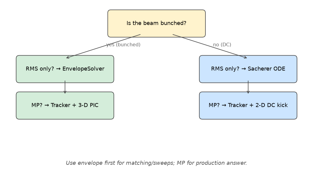
Figure 2.3 — Picking the right tracker for your physics regime.