Coordinates & units
Every quantity HELIX manipulates lives in a single, consistent coordinate system. This page is the contract: if you ever wonder "what units does this number have?" — the answer is here.
TL;DR
- 6-D phase space: (x, x', y, y', Δφ, ΔW)
- Units: mm, mrad, mm, mrad, deg, MeV
- Reference: x' = pₓ/p_z (kinetic, not canonical pₓ/p₀)
- Δφ: phase relative to the synchronous reference particle at the current RF frequency (changes at FREQ jumps)
- Emittance: ε reported in mm·mrad (geometric); ε_n = β·γ·ε (normalised) also recorded
- σ-matrix: 6×6, units (mm, mrad, mm, mrad, deg, MeV) on the diagonal
The 6-D state vector
Every particle carries a 6-component state. Indexing is consistent
across the codebase (Beam.particles[i, k] for k=0..5):
| Index | Symbol | Meaning | Units |
|---|---|---|---|
| 0 | x | transverse horizontal position | mm |
| 1 | x' | transverse divergence dx/dz = pₓ/p_z | mrad |
| 2 | y | transverse vertical position | mm |
| 3 | y' | transverse divergence dy/dz = p_y/p_z | mrad |
| 4 | Δφ | RF phase deviation from reference | deg |
| 5 | ΔW | kinetic energy deviation from reference | MeV |
This is TraceWin's reduced phase space. Three notes:
-
x' is kinetic, not canonical. HELIX uses x' = pₓ/p_z, not the canonical pₓ/p₀ used by some codes (e.g. MAD-X). Under solenoid coupling, the projected ε_x and ε_y oscillate; the 4-D invariant √det(σ_4D) and the symplectic normal-mode emittances ε₁, ε₂ stay constant. See Emittances for the full story.
-
Δφ is at the local RF frequency. In a multi-section linac (PIP-II: 162.5 → 325 → 650 MHz), Δφ at the same physical bunch length doubles or quadruples at each FREQ jump. This is the TraceWin convention. HELIX reports σ_φ at the local frequency too — see the convention note in PIP-II validation.
-
ΔW is energy, not momentum. Some codes use Δp/p₀. Conversion for small deviations: Δp/p = ΔW / (β²·γ·m·c²). (Derivation: E² = (pc)² + (mc²)² ⇒ dE = β·c·dp ⇒ dp/p = dE/(p·β·c) = ΔW/(γ·β²·m·c²).)
Lengths and longitudinal coordinates
| Quantity | Symbol | Units | Notes |
|---|---|---|---|
| Lattice path length | s | mm | accumulated along the design orbit |
| Element length | L | mm | TraceWin convention (also mm) |
| Reference frequency | f | MHz | BeamConfig.frequency, Lattice FREQ card |
| Synchronous phase | φ_s | deg | with respect to RF zero crossing |
| Bunch length | σ_z | mm | σ_z = β·c / (2π·f) · (σ_φ in rad) |
s in mm vs m
HELIX records results.s in mm to keep all transverse and
longitudinal lengths in one unit system. When plotting against
real machines it's common to convert to metres for axis labels:
s_m = np.asarray(results.s) / 1e3.
Reference particle
The ReferenceParticle carries the design orbit's instantaneous
state:
| Attribute | Meaning | Units |
|---|---|---|
species |
particle type (PROTON, H_MINUS, DEUTERON, …) | — |
w_kin |
kinetic energy | MeV |
frequency |
RF frequency at this point | MHz |
phi_s |
synchronous phase | deg |
beta |
β = v/c | — |
gamma |
γ = (1 + W/mc²) | — |
bg |
β·γ (normalised-emittance scaling) | — |
beta, gamma, bg are computed from w_kin + species mass; they
update whenever the reference particle traverses an accelerating
element. All transverse-plane optics depend on the running bg.
Emittance conventions
- Geometric ε_x = √(⟨x²⟩·⟨x'²⟩ − ⟨x·x'⟩²) (mm·mrad)
- Normalised ε_nx = β·γ · ε_x (mm·mrad)
- Longitudinal ε_z = √(⟨Δφ²⟩·⟨ΔW²⟩ − ⟨Δφ·ΔW⟩²) (deg·MeV)
- Normalised ε_nz = β·γ · ε_z(mm·mrad), where ε_z(mm·mrad) converts (deg, MeV) into (mm, mrad) via the local k_φ = 360°/(β·λ_RF). See Emittances.
BeamConfig.emit_nx is normalised
BeamConfig.emit_nx, emit_ny are normalised emittances. The
factory divides by the reference β·γ to produce the geometric
emittance the envelope solver expects. This is the most common
source of "factor of 11" σ overshoots at LEBT entrance — make
sure you're feeding normalised values to BeamConfig.
σ-matrix
The 6×6 covariance matrix Σ has the layout
Σ = | <xx>    <xx'>   <xy>    <xy'>   <xφ>    <xW>   |
    | <x'x>   <x'x'>  <x'y>   <x'y'>  <x'φ>   <x'W>  |
    | <yx>    <yx'>   <yy>    <yy'>   <yφ>    <yW>   |
    | <y'x>   <y'x'>  <y'y>   <y'y'>  <y'φ>   <y'W>  |
    | <φx>    <φx'>   <φy>    <φy'>   <φφ>    <φW>   |
    | <Wx>    <Wx'>   <Wy>    <Wy'>   <Wφ>    <WW>   |
with diagonal-element units (mm², mrad², mm², mrad², deg², MeV²). Σ[0, 0] = σ_x², Σ[2, 2] = σ_y², Σ[4, 4] = σ_φ², etc.
The full Σ is recorded per-step on DiagnosticRecorder.sigma_matrix
and is the basis for every Twiss / emittance / eigenemittance
diagnostic.
What is not tracked
- Time t — the simulation is parameterised by s, not t. Time is recovered if needed from t = ∫ ds / (β·c).
- Particle flavour or charge state changes mid-flight — H⁻ stripping is computed as a post-tracking analyser (H⁻ stripping), not as a state transition.
- Quantum / spin states — irrelevant for the proton-linac use case.
Diagram
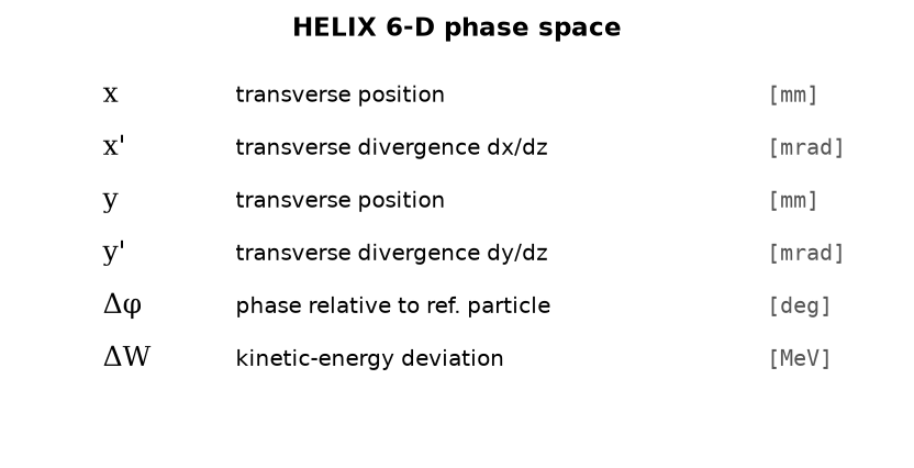
Figure 2.1 — HELIX 6-D phase space. The first four components describe the transverse plane (kinetic divergence, not canonical momentum). The last two describe the longitudinal plane relative to a synchronous reference particle.
Cross-references
- Data model — how the Lattice, Beam, ReferenceParticle hold this data.
- Distributions — how particle states get initialised.
- Recorder fields — which arrays record which coordinates.