Distributions¶

HELIX ships six particle distribution generators, plus file loading (source="file"). Pick the one that best models your physical situation; the choice affects σ prediction, halo, and aperture-loss results.

TL;DR — pick one¶

Distribution	Density profile	Use case
waterbag (default)	uniform 6-D ellipsoid	textbook benchmark; ~Gaussian RMS but no tails
gaussian	exp(-r²/2σ²), truncated at `cutoff·σ`	most realistic for production beams
kv	Kapchinskij-Vladimirskij (uniform charge density)	analytic envelope solutions
parabolic	parabolic transverse density	TraceWin compatibility; matches partran's option
uniform	uniform cube in normalised phase space	extreme stress test; never realistic
thermal	bi-Gaussian core + halo	PIP-II realistic; halo extends beyond the core cutoff

To load a beam from disk instead of generating one, set source="file" + distribution_file (TraceWin .dst binary or ASCII text) — see File loading below.

Tutorial¶

All distributions are accessed via BeamConfig.distribution and create_beam(config, seed):

from linac_gen.core.config import BeamConfig
from linac_gen.distributions.factory import create_beam

# Same Twiss + emittance + species; only the distribution differs
common = dict(
    species="proton", energy=3.0, frequency=352.21,
    current=5.0, n_particles=10_000,
    emit_nx=0.25, emit_ny=0.25, emit_z=0.30,
    alpha_x=0.0, beta_x=2.0,
    alpha_y=0.0, beta_y=2.0,
    alpha_z=0.0, beta_z=1.0,
)

beam_g = create_beam(BeamConfig(distribution="gaussian", cutoff=4.0,  **common))
beam_w = create_beam(BeamConfig(distribution="waterbag",              **common))
beam_t = create_beam(BeamConfig(distribution="thermal",
                                halo_fraction=0.05, halo_ratio=5.0,    **common))

All produce particles matching the requested ε, α, β at second-moment level — the difference is in the higher moments.

Distribution details¶

Gaussian¶

Truncated at cutoff × σ (default 3.0) to avoid unrealistic outliers; raise the cutoff (e.g. 4.0-6.0) for halo-aware studies. The same cutoff field also truncates the thermal core.

Waterbag¶

Uniform inside a 6-D ellipsoid in (x, x', y, y', φ, W) space. RMS matches a Gaussian with the same ε but the tails are sharply cut off — every particle is within an envelope. Useful for benchmark comparisons and matching tests.

Kapchinskij-Vladimirskij (KV)¶

Uniform transverse charge density, uniform momentum distribution (δ-function on the boundary of the 4-D ellipsoid). Self-consistent with linear envelope dynamics — the only non-trivial distribution that gives exactly linear space-charge forces. Used in textbook derivations.

Parabolic¶

Parabolic transverse density ρ(r) ∝ (1 - r²/r_max²) for r < r_max. Matches a TraceWin partran option and produces somewhat softer tails than waterbag.

Uniform¶

Uniform cube in normalised phase space. Extreme; useful only as a stress test.

Thermal (bi-Gaussian halo)¶

A Gaussian core with halo_fraction of the particles drawn from a secondary, wider Gaussian (halo_ratio × σ). Renormalised so the combined RMS matches the requested ε. Models PIP-II's measured halo content far better than a single Gaussian; necessary for accurate aperture-loss prediction in long beamlines.

beam_cfg = BeamConfig(
    distribution="thermal",
    halo_fraction=0.05,    # 5% of particles in the halo
    halo_ratio=5.0,        # halo at 5σ width
    # ... other params
)

File loading (`source="file"`)¶

Loading a beam from disk is not a distribution — it is a separate source path selected by source="file" (the distribution field is ignored). Two formats:

.dst — TraceWin binary format. Header carries energy, frequency, ε, Twiss, current — these override the BeamConfig fields when source="file".
anything else — ASCII text: six whitespace-separated columns x(mm) xp(mrad) y(mm) yp(mrad) phi_abs(deg) W_abs(MeV), with optional # w_kin_ref: / # phi_ref: header lines. (There is no HDF5 loader.)

The factory uses the file's full particle count — there is no subsampling, and n_particles is ignored for file sources:

beam_cfg = BeamConfig(
    species="proton",
    source="file",
    distribution_file="examples/lebt_pxie/initial_beam.dst",
)

For full .dst details see .dst loading.

Visual comparison¶

Distribution gallery

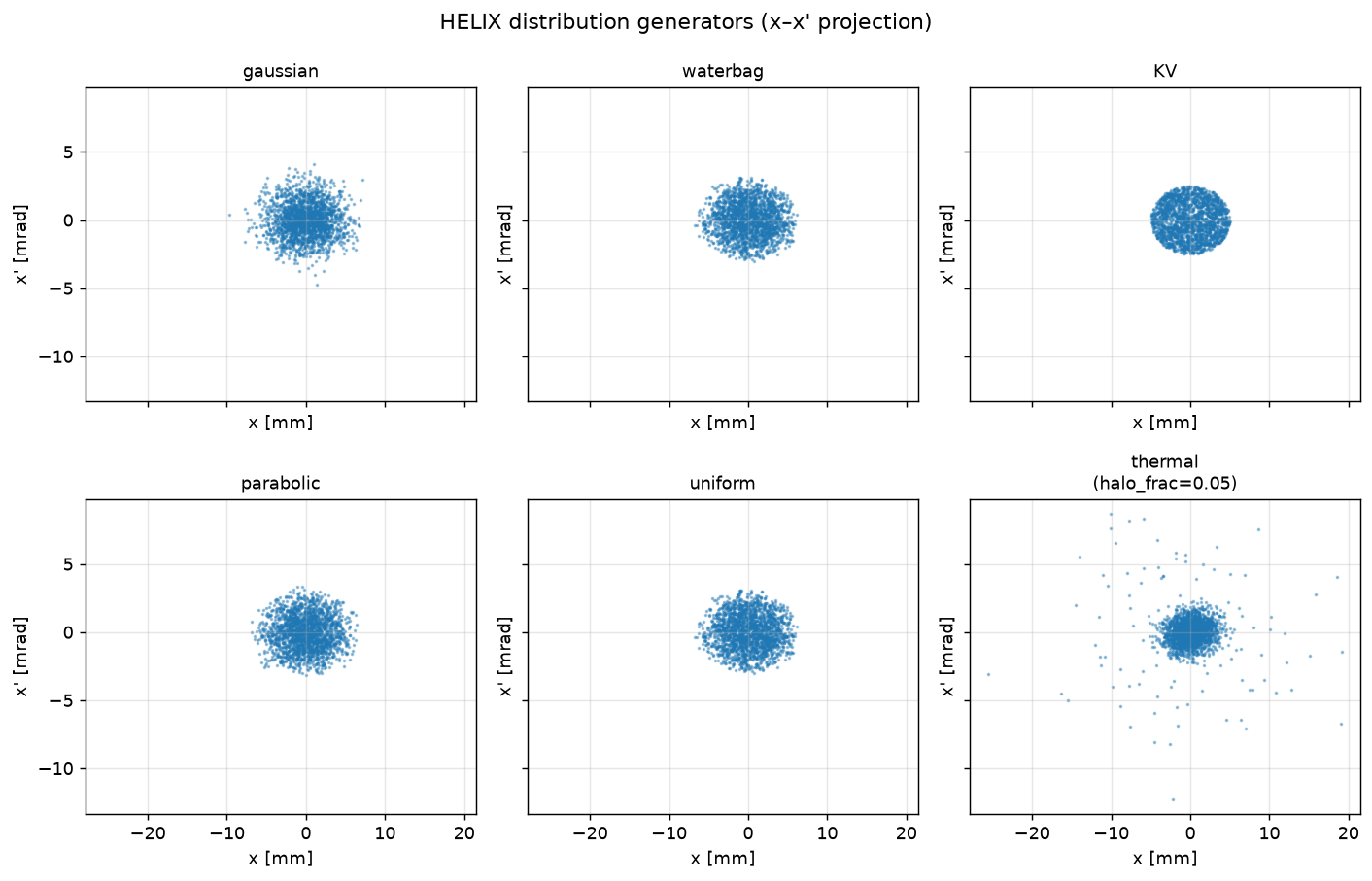
Figure 4.1 — x-x' projections of the six built-in distributions, all matched to the same Twiss (β_x = 2.0 m, ε_n = 0.25 mm·mrad). Note how the cores look similar at the σ level but the tails differ: gaussian has the longest tail, KV is hard-cut, thermal has explicit halo content.

API reference¶

linac_gen.distributions.factory.create_beam(
    config: BeamConfig,
    seed: int | None = None,
) -> Beam

seed is forwarded to the underlying distribution generator — None draws from system entropy.

Source¶

linac_gen/distributions/factory.py:1
linac_gen/distributions/{gaussian,waterbag,kv,parabolic,uniform,thermal,from_file}.py